Gaussian curvature
Definition 1
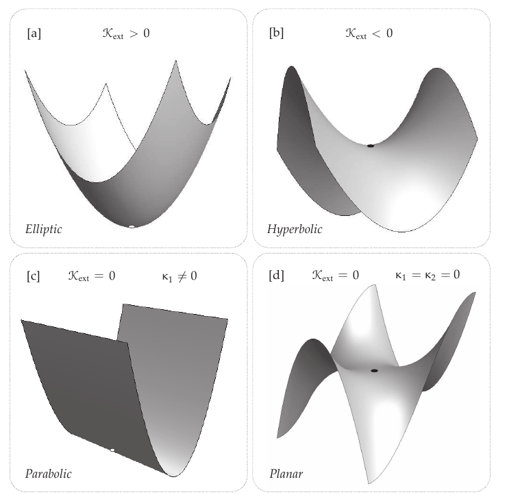
The Gaussian curvature is the product of the principal curvatures:
$$ \mathcal{K}=\kappa_1 \cdot \kappa_2 \tag{1} $$In this sense, it is the determinant of the shape operator.
Picture from @needham2021visual page 136 (he calls it $\mathcal{K}_{ext}$)
Definition 2
It is the local area magnification of the Gauss map
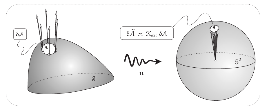
(@needham2021visual page 132)
Sometimes it is called extrinsic curvature.
Definition 3
At a point $p$, $\mathcal{K}(p)$ can be defined as the local angular excess per unit area (@needham2021visual page 18):
$$ \mathcal{K}(p)=\lim _{\Delta_{p} \rightarrow p} \frac{\mathcal{E}\left(\Delta_{p}\right)}{\mathcal{A}\left(\Delta_{p}\right)} $$Here $\mathcal{E}(\Delta)$ is the sum of the angles of the triangle $\Delta$ minus $\pi$. This is rather informal, but I think it can be formalized as the angle defect of parallel transport about a geodesic triangle. It is related to Harriot theorem. Also related to the local Gauss-Bonnet theorem.
Equivalences of definitions (incomplete)
See this question and this answer in mathoverflow.
- Proving that definition 1 and definition 2 are equivalents is easy. A visual aid is in @needham2021visual page 134
- To visualize the equivalence of definition 2 and 3:
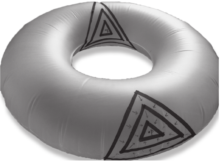
There is a physical "proof" of this fact which I learned from Mark Levy; it is in his book "THE MATHEMATICAL MECHANIC: Using Physical Reasoning to Solve Problems".
Imagine that you keep the axis of a bicycle wheel and move it in such a way that the bicycle wheel lies in the tangent plane to the surface. In the initial position the wheel stays still; you go along a loop in the surface and stop. After that your wheel rotates by some angle α with respect to the initial position. If your loop was triangular this angle is its defect; this is definition 3.
The parallel motion does not rotates the wheel, so the same result will be the same if you only rotate the axis without moving the center of the wheel. This tells you that α depends only on the spherical image of the loop and from here it is easy to see that it is proportional to the algebraic area of the domain bounded by the spherical image of the loop. I.e., the area of the sphere that Gauss map traces out on a region; this is definition 2.
- Equivalence between 1 and 3 is done, visually, in @needham2021visual page 256.
Facts
1. To compute it we can use the first fundamental form and the second fundamental form. Coming from notation here, we have
$$ \begin{aligned} K &=\operatorname{det}\left(\mathcal{F}_{1}^{-1} \mathcal{F}_{2}\right) \\ &=\operatorname{det}\left(\mathcal{F}_{1}\right)^{-1} \operatorname{det}\left(\mathcal{F}_{2}\right) \\ &=\frac{L N-M^{2}}{E G-F^{2}} . \end{aligned} $$It is not strange that we use the second fundamental form if we take into account Definition 1 and Definition 2 (extrinsic definitions).
2. But surprisingly enough, it does not depend on the second fundamental form, is an intrinsic property! This can be observed in definition 3. This was stated by Gauss in his Theorema Egregium. This can also be concluded by (or it is used in) the local Gauss-Bonnet theorem.
4. Therefore, it can be computed only with the first fundamental form. In an orthogonal coordinate system (i.e., $F=0$) we have:
$$ K=-\frac{1}{2 \sqrt{E G}}\left(\frac{\partial}{\partial u} \frac{G_{u}}{\sqrt{E G}}+\frac{\partial}{\partial v} \frac{E_{v}}{\sqrt{E G}}\right) $$Following notation introduced here it can be computed with
$$ \mathcal{K}=-\frac{1}{A B}\left(\partial_{v}\left[\frac{\partial_{v} A}{B}\right]+\partial_{u}\left[\frac{\partial_{u} B}{A}\right]\right) $$This is called the metric curvature formula. It is shown in @needham2021visual page 268, by using the holonomy#Local chart and the fact that the curvature is ultimately equal to the holonomy per unit area. But it also appears in @needham2021visual page 452 by using Cartan's method of moving frames.
5. Gaussian curvature has a simpler expression in isothermal coordinates.
6. Non orthogonal coordinates. According to Wikipedia page, we have the Brioschi formula
$$ K=\frac{\left|\begin{array}{ccc} -\frac{1}{2} E_{v v}+F_{u v}-\frac{1}{2} G_{u u} & \frac{1}{2} E_u & F_u-\frac{1}{2} E_v \\ F_v-\frac{1}{2} G_u & E & F \\ \frac{1}{2} G_v & F & G \end{array}\right|-\left|\begin{array}{ccc} 0 & \frac{1}{2} E_v & \frac{1}{2} G_u \\ \frac{1}{2} E_v & E & F \\ \frac{1}{2} G_u & F & G \end{array}\right|}{\left(E G-F^2\right)^2} $$7. It is related to geodesics by means of Jacobi equation.
8. The total curvature in a region $\Omega$ coincides with the holonomy of the loop $\partial \Omega$. See @needham2021visual page 246
Visualizations:
Angular excess
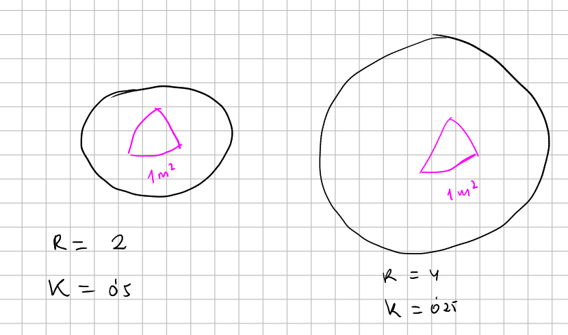
I think that from the local Gauss-Bonnet theorem can be deduced, in a constant curvature surface:
$$ K=\frac{\mathcal{E}(\Delta)}{\mathcal{A}(\Delta)} $$where $\Delta$ is a triangle made of geodesics, $\mathcal{E}(\Delta)$ is the angular excess $\sum \alpha_i-\pi$, and $\mathcal{A}(\Delta)$ is the area of this triangle. Imagine a triangle of unit area painted on a sphere, it will have an angular excess given, visually, by the non-straightness of the edges. If we inflate the sphere we obtain a surface with less curvature, and a triangle with the same area will be then, relatively, smaller, and the edge will look more straight (less angle excess)
If the surface is not of constant curvature for a point $p$:
$$ K_p=\lim_{\Delta_p \to p} \frac{\mathcal{E}(\Delta_p)}{\mathcal{A}(\Delta_p)} $$where $\Delta_p \to p$ means that we have a succession of triangles shrinking down toward $p$. See [Needham 2021].
This can be generalized to $n$-gon with
$$ \mathcal{E}(n-g \circ n) \equiv[\text { angle sum }]-(n-2) \pi, $$Area excess
From wikipedia.
Gaussian curvature is the limiting difference between the area of a geodesic disk and a disk in the plane
$$ K=\lim _{r \rightarrow 0^{+}} 12 \frac{\pi r^{2}-A(r)}{\pi r^{4}} $$The particular case of a sphere: @needham2021visual page 20. Proof in general: @needham2021visual page 278.
Length excess
Gaussian curvature is the limiting difference between the circumference of a geodesic circle and a circle in the plane
$$ K=\lim _{r \rightarrow 0^{+}} 3 \frac{2 \pi r-C(r)}{\pi r^{3}} $$The particular case of a sphere: @needham2021visual page 20, again. Proof in general: @needham2021visual page 278.
Relation to the curvature of a connection
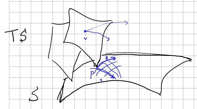
What follows is a very informal annotation.
Consider a surface $S$ and the tangent space $TS$. The Riemannian metric of $S$, i.e., the first fundamental form, let us define the Levi-Civita connection which, at the end of the day, is a distribution on $TS$, that is, a subbundle of $T(TS)$. How is this? Well, given a vector $v\in T_p S$, parallel transport let us define two "infinitesimal curves" in $TS$ leaving $v$, being one of them the parallel transport along the first coordinate direction $x$ and the other the parallel transport along the second coordinate direction $y$. These two curves are transversal to $V$, the vertical subbundle of $T(TS)$, because we are leaving $p$, and let us take their tangent vectors to define a subvector space of $T_v TS$: the horizontal space of the distribution-connection, in such a way that $T(TS)=V\oplus H$.
The curvature of this connection (in the sense of performing the bracket of the vector fields of the horizontal distribution and then project to the vertical distribution) should be the same as the Gaussian curvature of the surface or, at least, be directly related. For example, observe that if the surface has non-zero Gaussian curvature, then parallel transports do not, in general, commute. This corresponds to the fact that $H$ does not posses integral manifolds, because if we leave $v$ travelling along curves tangent to $H$ (parallel transports) we may arrive to a different $v'\in T_pS$. In other words, flat surfaces (in the sense of Gaussian curvature) let us create copies of it in every $v$, so we can foliate $TS$ with these copies.
More formally
In a Riemannian surface $(S,g)$ consider the Levi-Civita connection $\nabla$ corresponding to the metric $g$. Suppose we have an orthonormal frame $\{e_1,e_2\}$ with dual coframe $\{\omega^1,\omega^2\}$. We know that $\nabla$ is described here by the connection forms
$$ \Theta=\begin{pmatrix} 0&-T_{12}^1 \omega^1-T_{12}^2\omega^2\\ T_{12}^1 \omega^1+T_{12}^2 \omega^2&0\\ \end{pmatrix}, $$where $d\omega^1=T_{12}^1 \omega^1 \wedge \omega^2$ and $d\omega^2=T_{12}^2 \omega^1 \wedge \omega^2$ (see here).
The curvature of the connection is a matrix of 2-forms $\Omega=d\Theta$. Indeed, by mere computations we arrive to
$$ \Omega=-\left(e_1(T_{12}^2)-e_2(T_{12}^1)+(T_{12}^1)^2+(T_{12}^2)^2\right)\begin{pmatrix} 0& \omega^1 \wedge \omega^2\\ -\omega^1 \wedge \omega^2&0\\ \end{pmatrix}. $$Gauss equation says that
$$ d\Theta^1_2=K \omega^1 \wedge \omega^2 $$(@ivey2016cartan page 47). Then $d\Theta^1_2(e_1,e_2)=-\left(e_1(T_{12}^2)-e_2(T_{12}^1)+(T_{12}^1)^2+(T_{12}^2)^2\right)$ is indeed the Gaussian curvature of the surface.
Proof of Gauss equation
Let's see it for an immersed surface $\iota:S\to \mathbb{R}^3$ (also in @needham2021visual section 38.5.1). We consider a point $p\in S$ and an open neighbourhood $U\subset \mathbb R^3$ of $p$. We have the unit normal vector to the surface $n$, and think of a orthonormal frame $\{\tilde{e}_1,\tilde{e}_2,\tilde{n}\}$ defined on $U$ such that gives rise to $\{e_1,e_2,n\}$ when restricted to $S$. Analogously, we have the dual coframe $\{\tilde{\omega}_1,\tilde{\omega}_2,\tilde{\zeta}\}$. We can compute here the connection 1-forms matrix $\tilde{\Theta}$ of the standard connection $\nabla_{std}$ with respect to this frame (see this). It turns out that
$$ \tilde{\Theta}= \left(\begin{array}{cccc} 0 &\tilde{\Theta}_2^1 & \tilde{\Theta}_3^1 \\ -\tilde{\Theta}_2^1& 0& \bar{\Theta}_3^2 \\ -\bar{\Theta}_3^1 & -\bar{\Theta}_3^2 & 0 \end{array}\right) $$where it is satisfied that $\iota^*(\tilde{\Theta}_2^1)={\Theta}_2^1$. To see this, observe that on the one hand we have
$$ \nabla_V e_2=V\lrcorner \Theta^1_2 e_1, $$and in the other, since $\nabla$ is the induced connection by the standard metric in $\mathbb R^3$,
$$ \nabla_V e_2=\mbox{proj}((\nabla_{std})_V \tilde{e}_2)=\mbox{proj}(V\lrcorner \tilde{\Theta}^1_2\tilde{e}_1-V\lrcorner \tilde{\Theta}^2_3 \tilde{n})=V\lrcorner \iota^*(\tilde{\Theta}^1_2)e_1 $$for an arbitrary vector $V$ tangent to $S$.
Now, we have to put together several things:
- First, we know that Gaussian curvature $K$ is the determinant of the shape operator.
- Second, it turns out that this determinant can be computed as $\tilde{\Theta}^1_3 \wedge \tilde{\Theta}^2_3(e_1,e_2)$ (see here to see why) evaluated in points $p$ of the surface $S$.
- Then, according to Cartan's second structural equation, since $\mathbb R^3$ is flat
and then
$$ d\tilde{\Theta}^1_2=\tilde{\Theta}^3_2\wedge \tilde{\Theta}^1_3 $$an
$$ d\tilde{\Theta}^1_2(e_1,e_2)=\tilde{\Theta}^3_2\wedge \tilde{\Theta}^1_3(e_1,e_2)=-\tilde{\Theta}^1_3\wedge \tilde{\Theta}^3_2(e_1,e_2)=\tilde{\Theta}^1_3\wedge \tilde{\Theta}^2_3(e_1,e_2) $$If we restrict this identity to $S$ we obtain
$$ d{\Theta}^1_2(e_1,e_2)=K. $$Pending task: I want to describe all latter stuff with the method of moving frames. I think I can show that $K$ is one of the invariants provided by the MC form, but for the elements of Euclidean group $E(3)$. So $K$ is invariant under congruence (like median curvature, I guess). But I don't know yet how to show it for general isometries of the surface. It is maybe explained here. May is also interesting this paper of Chern. (See also @ivey2016cartan page 47)
Maybe this is also related to what is said in Generalization of the flatness of R3.
________________________________________
________________________________________
________________________________________
Author of the notes: Antonio J. Pan-Collantes
INDEX: